The limnopapers twitter feed underwent a comprehensive revamp in December 2018. I replaced the click-based framework detailed by Rob Lanfear here with a custom scripted solution using a feedparser and python-twitter backend. Rather than tediously adding include and exclude keywords through a web gui and being limited to 5 feeds, this new solution allows easy control over keywords and tracking as many feeds as you want. In addition to custom feed handling in the new system (I can now deal with feeds that come in a variety of formats instead of being limited to the dlvr.it parser) there is a built-in system for logging tweets that have passed through the keyword filters and can be considered “limnology papers”.
In the following post, I take a look at this log to to get a sense of Limnology in 2019.
import pandas as pd
import seaborn as sns
import wordcloud
log_raw = pd.read_csv("log.csv")log = (log_raw
.loc[log_raw["posted"] == "y"])
log["date"] = pd.to_datetime(log["date"])First, lets look at the top papers of the year as measured by twitter likes:
AquaSat: a dataset to enable remote sensing of water quality for inland waters. Water Resources Research. https://t.co/RNxifhH0qi
— limnopapers (@limno_papers) October 14, 2019
Large spatial and temporal variability of carbon dioxide and methane in a eutrophic lake. Journal of Geophysical Research: Biogeosciences. https://t.co/uHyTN6xT4b
— limnopapers (@limno_papers) July 3, 2019
Process‐guided deep learning predictions of lake water temperature. Water Resources Research. https://t.co/h8rBDbVaKy
— limnopapers (@limno_papers) November 11, 2019
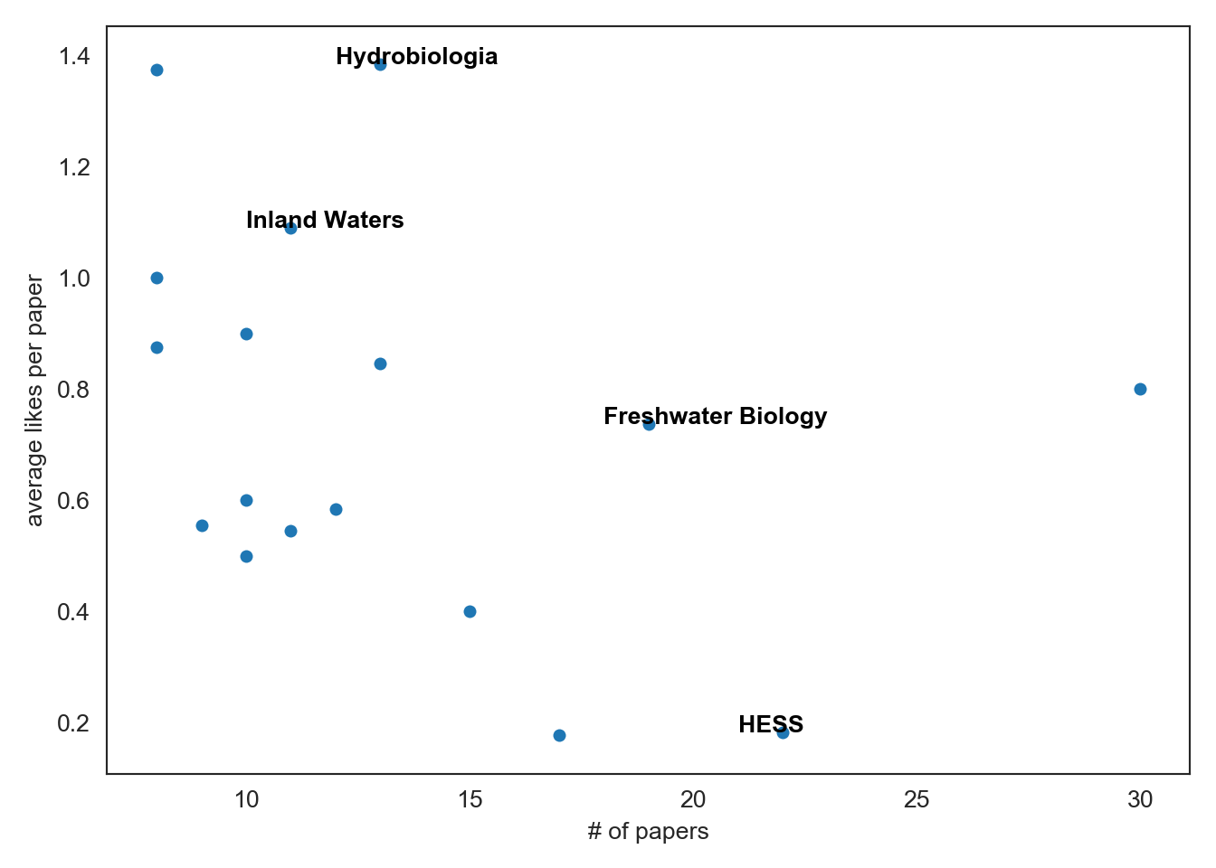
Next, lets look at the top journals of the year as measured by number of papers and average likes per paper. Looks like Water Resources Research is leading the pack with the most limnopapers in 2019 but Hydrobiologia papers are getting the most likes.
log_perjournal = (log
                  .groupby(["dc_source"])
                  .agg(["count"])
                  .reset_index()
                  .iloc[:, 0:2])
log_perjournal.columns = ["dc_source", "count"]
log_perjournal = log_perjournal.sort_values(by = ["count"], ascending = False)

sns.barplot(data = log_perjournal.query("count > 6"), y = "dc_source", x = "count")
plt.xlabel("count")
plt.ylabel("")
plt.tight_layout()
plt.show()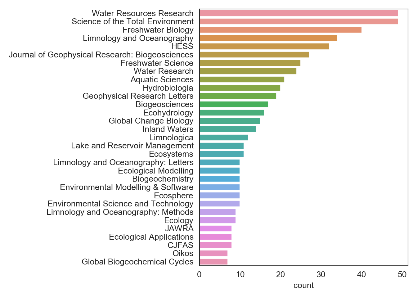
Next, lets look at a wordcloud of paper titles to see common themes:
wc = wordcloud.WordCloud().generate(log["title"].str.cat(sep=" "))
plt.imshow(wc)
plt.show()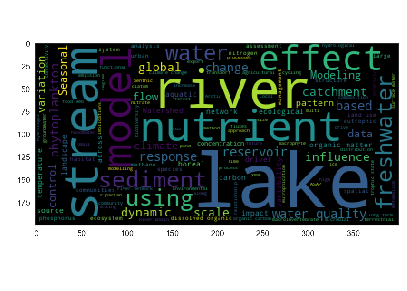
To wrap things up, lets look at a cumulative timeline of limnopapers tweets. We saw about 600 papers in 2019.
log_cumsum = (log
              .groupby(["date"])
              .agg(["count"])
              .loc[:, ["date", "title"]]
              .cumsum())

chart = (log_cumsum
         .pipe((sns.lineplot, "data"))
         .legend_.remove())
plt.xlabel("")
plt.ylabel("Cumulative tweets")
plt.tight_layout()
plt.show()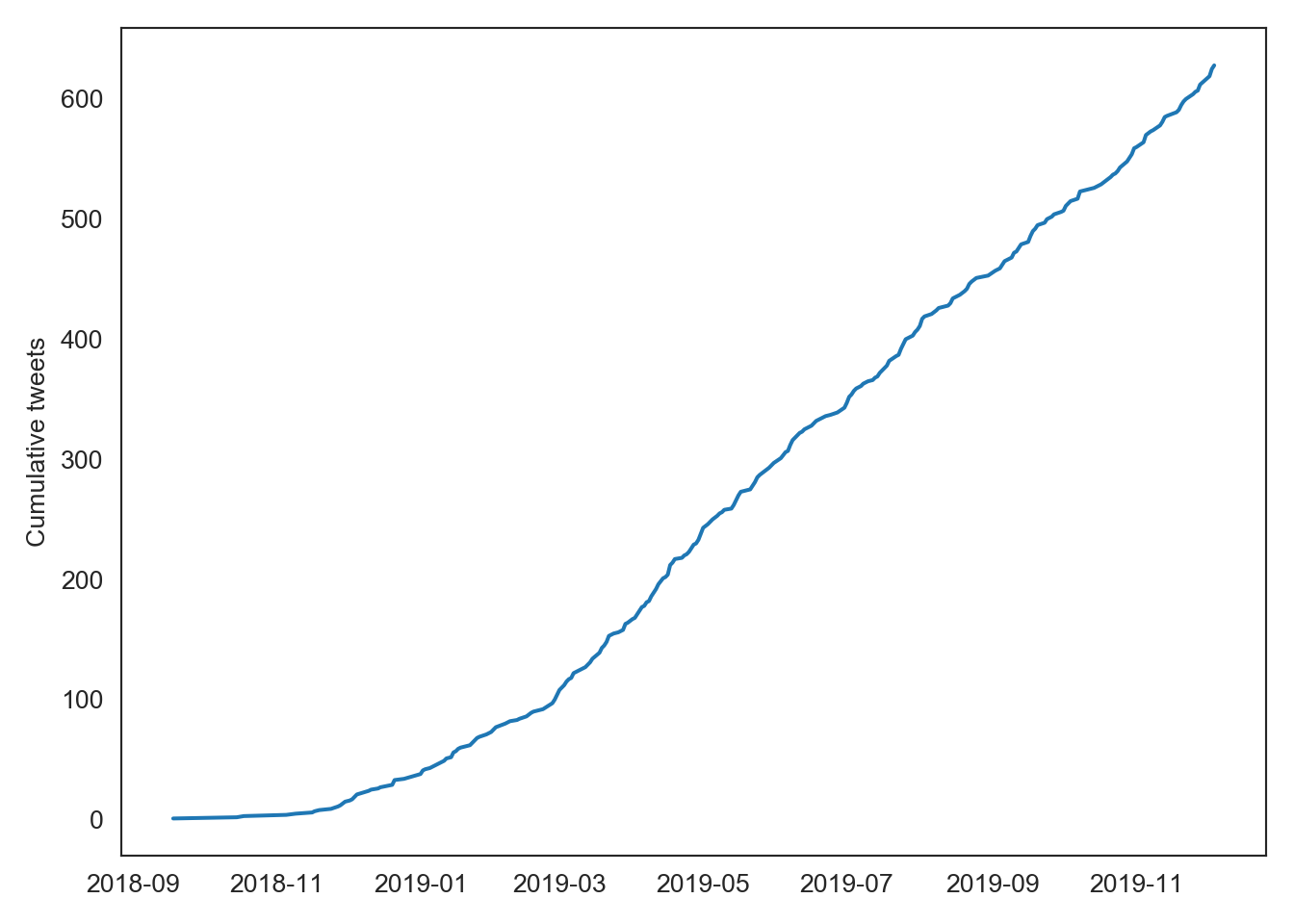
…and there was no real pattern in the day of the week when most papers are posted. Looks like Friday is the most popular day followed closely by Tuesday.
# per day stats
# calculate day of the week from date, group per day and sum
log['day_of_week'] = log['date'].dt.day_name()
days = ['Monday', 'Tuesday', 'Wednesday', 'Thursday', 'Friday']

log_perday = (log
              .groupby(["day_of_week"])
              .agg(["count"])
              .loc[:, ["title"]]
              .reset_index()
              .iloc[:, 0:2])
log_perday.columns = ["day", "count"]

log_perday = log_perday[~log_perday["day"].isin(["Saturday", "Sunday"])]
log_perday.day = log_perday.day.astype("category")
log_perday.day.cat.set_categories(days, inplace=True)
log_perday = log_perday.sort_values(["day"])

sns.barplot(data = log_perday, y = "day", x = "count")
plt.tight_layout()
plt.show()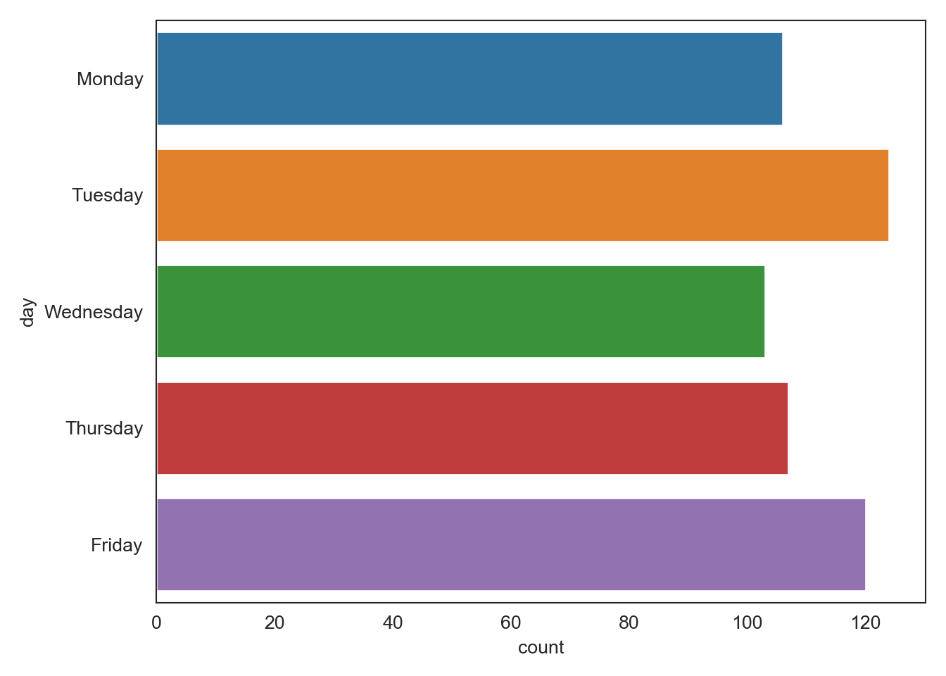
Certainly caveats apply here. My keyword choices reflect a specific interpretation of limnology, my journal choices are limited to only a few dozen titles, and I used my personal judgement to tune the papers that were posted. Anyone interested in running their own feed either on limnology or some other topic can do so by forking the code at https://github.com/jsta/limnopapers and adjusting the feed choices in feeds.csv and/or the keywords in keywords.csv.